The CLT
The Central Limit Theorem (CLT) answers an important question: Why does the bell curve (the Normal Distribution) show up everywhere in the real world?
More specifically, the theorem describes what happens when we take a random variable, say \(X\), and repeat any “experiment” many times to get a series of outcomes (resulting output values of the random variable), \(X_1, X_2, \dots, X_m\). What does the distribution of their sum (\(S_m = X_1 + \dots + X_m\)) or their average (\(\bar{X}_m = S_m/m\)) look like when \(m\) is very large?
For the bell curve phenomenon to happen, the random variables must be IID (Independent and Identically Distributed).
- Independent: The outcome of one trial of the experiment doesn’t influence the next (the die has no memory).
- Identically Distributed: We’re drawing from the same random process every time (e.g., rolling the same die with the same probability distribution).
When these conditions are met, the Central Limit Theorem states that the distribution of the sum (or average) will converge to a curve as the number of trials \(m\) becomes larger and larger.
What makes this profound and useful though is its universality. It doesn’t matter what the probability distribution of the original variable \(X\) is. We could be rolling an ordinary six-sided die, tossing a biased coin, or measuring something with a weird, skewed distribution that looks nothing like a bell curve. The result is always the same: after summing enough of them, the bell curve emerges naturally.
We see this everywhere:
- Human Height: The height of a single person is determined by a large number of random factors: genetics, nutrition, and so on. The final height of a single person (the random variable in this case) may be a complicated function of these factors, and may not be a normal distribution. Still when the sum of heights for a large number of different individuals is taken, this sum (and thus the average height) results in the classic bell-curve distribution of heights we see in the population.
- Manufacturing: The number of microscopic flaws in a single semiconductor chip might follow some unknown distribution dependent on the manufacturing process and other factors. But the total number of flaws in a batch of chips (say a 1000 chips) will, again, follow a bell curve, which is the basis for statistical quality control.
So essentially what happens is that individual randomness gets “averaged out” and a predictable shape emerges. The emergent bell curve only cares about the mean and variance of the original random variable \(X\), completely forgetting all other details of its probability distribution. The following derivation explains exactly why this phenomenon occurs.
Encoding Probabilities (The PGF)
To get to the heart of the Central Limit Theorem, we need a mathematical tool to describe what happens when we sum up many random variables, like the rolls of a die. Let’s try to build such a tool from first principles.
The challenge is this: when we add the scores from two dice, their outcomes should add, but their independent probabilities should multiply (by the laws of probability). How can we find a mathematical representation that encapsulates this behavior?
Let’s focus on the outcomes first. Suppose we represent an outcome value \(a\) by \(f(a)\). We want the combination of two outcomes \(a\) and \(b\) to correspond to the outcome \(a+b\). The “combination” of two outcomes entails a multiplication of their probabilities (only if the outcomes are independent). Thus our representation function \(f(x)\) needs to satisfy \(f(a)\,f(b)=f(a+b)\).
This functional equation is pretty common and has a well known solution which can be easily derived: \(f(a)=x^a\) for some base \(x\). We see that \(x^a x^b = x^{a+b}\), exactly as we require.
This gives us the key. We can represent an outcome \(k\) with the term \(x^k\). The variable \(x\) is just a placeholder. Now where do the probabilities fit in here? A probability \(p_k\) is the weight of the outcome \(k\), so the most natural place to put it is as a coefficient: \(p_k x^k\).
To represent the entire die, which can take on any of the values \(\{1, 2, 3, 4, 5, 6\}\), we can simply sum up these weighted terms. This creates a polynomial, which packages all the information about our random variable into a single expression. This representation is called the Probability Generating Function (PGF).
For a discrete random variable \(X\) that takes integer values with probabilities \(p_k=\Pr(X=k)\), we define its PGF as:
\[H(x)=\sum_k p_k\,x^k.\]
Before applying this representation to dice, a quick analogy from counting clarifies why polynomials are appropriate and convenient representations encoding probability distributions.
An analogy from counting
Let’s see this polynomial representation we discussed above in a simpler context: counting combinations. This idea is a cornerstone of combinatorics for solving counting problems.
Imagine we want to count the number of ways to form 10 Rupees using a collection of 1, 2, and 5 Rupee coins. This is a classic combinatorial problem. We can represent the available coins as polynomials:
- 1 Rupee Coins: \((1 + x^1 + x^2 + \dots)\)
- 2 Rupee Coins: \((1 + x^2 + x^4 + \dots)\)
- 5 Rupee Coins: \((1 + x^5 + x^{10} + \dots)\)
When we multiply these polynomials, voila! The coefficient of \(x^{10}\) in the final product gives we the exact number of ways to make change for 10 Rupees.
Why does this work? The exponents add, just like the coin values do. The polynomial multiplication automatically explores every single combination of choices for us. A PGF does the exact same thing, but the coefficients are probabilities instead of \(1's\) for counting.
Why is this a natural representation?
- Powers as labels: The exponent \(k\) is just a label for the outcome \(X=k\). The polynomial is in effect a storage system where the coefficient of \(x^k\) holds the probability of the outcome \(k\).
- Convolution by multiplication: This is the crux of why this representation works. If \(X\) and \(Y\) are independent, the probability that \(X+Y=n\) is found by summing over all pairs of outcomes that add to \(n\): \(\sum_k \Pr(X=k)\Pr(Y=n-k)\). This operation is called a convolution. When we multiply the PGFs \(H_X(x)\) and \(H_Y(x)\), the rule for multiplying polynomials does exactly the same calculation. The coefficient of \(x^n\) in the product is precisely that sum! So, for sums of independent variables, the PGF of the sum is the product of the PGFs: \[H_{X+Y}(x)=H_X(x)\,H_Y(x).\]
- From coins to dice: For a biased coin where heads \(=1\) and tails \(=0\), with \(\Pr(1)=p\), the PGF is \(H(x) = (1-p)x^0 + px^1\). For two flips, the PGF is \(H(x)^2 = (1-p)^2 + 2p(1-p)x^1 + p^2x^2\). The coefficients are simply the binomial probabilities. This idea extends perfectly to dice or any other discrete distribution.
For distributions that can take negative integer values, the PGF becomes a Laurent series with negative powers, like \(H(x) = \sum_{k=-\infty}^{\infty} p_k x^k\). All the logic, including the convolution property and the Cauchy integral extractor, works exactly the same!
Let’s now demonstrate this for a fair six-sided die. To match common conventions, we’ll switch the placeholder from \(x\) to \(z\) when we write the die’s blueprint \(h(z)\) and use coefficient extraction \([z^n]\).
For a standard fair die, the outcomes are \(\{1, 2, 3, 4, 5, 6\}\), each with probability \(\tfrac{1}{6}\). The representation function is: \[ h(z) = \frac{1}{6}z^1 + \frac{1}{6}z^2 + \frac{1}{6}z^3 + \frac{1}{6}z^4 + \frac{1}{6}z^5 + \frac{1}{6}z^6 \]
The Magic of Multiplication
What if we want the probabilities for the sum of two dice? We simply multiply the representation function by itself: \(h(z)^2\).
Why does this work? Consider getting a total of 3. This can happen as (1+2) or (2+1). When we multiply out \(h(z) \times h(z)\), this automatically finds every combination that produces a \(z^3\) term: \[ \underbrace{\left(\tfrac{1}{6}z^1\right) \times \left(\tfrac{1}{6}z^2\right)}_{\text{Roll 1, then 2}} + \underbrace{\left(\tfrac{1}{6}z^2\right) \times \left(\tfrac{1}{6}z^1\right)}_{\text{Roll 2, then 1}} = \frac{2}{36}z^3 \]
The resulting expression does all the tedious bookkeeping for us! The coefficient \(\tfrac{2}{36}\) is exactly the correct probability for the sum being 3.
This powerful idea is our starting point: To find the probability that the sum of \(m\) rolls is \(n\), we just need to find the coefficient of the \(z^n\) term in the expansion of \(h(z)^m\). We write this as \([z^n]h(z)^m\).
A worked example (three dice)
Let \(h(z)=\tfrac{1}{6}(z+z^2+z^3+z^4+z^5+z^6)\). For three dice, \[ [z^9]h(z)^3 = \sum_{a+b+c=9} \tfrac{1}{6^3}\,1 = \frac{25}{216}, \] where the \(25\) solutions \((a,b,c)\in\{1,\dots,6\}^3\) with \(a+b+c=9\) are counted by by direct enumeration. This matches the usual table of sums for three dice.
Notation: the coefficient operator
For a formal power series \(F(z)=\sum_n c_n z^n\), the extractor is \[[z^n]F(z)=c_n.\] When \(F\) is analytic on and inside a circle \(\gamma\), Cauchy’s formula gives an integral representation of this operator (next section).
The “Coefficient Extractor” Machine
Why do we need an extractor?
For a small number of dice, say \(m=3\), we could grit our teeth and manually expand the polynomial \(h(z)^3\) to find the probability of any given sum. But for \(m=100\), this is practically impossible. The polynomial would have hundreds of terms, and we only care about one of them! We need a surgical tool, a mathematical machine that can reach out into the enormous expansion of \(h(z)^m\) and pull out just the single coefficient we need, \([z^n]h(z)^m\), without doing the whole expansion.
How to Isolate a Coefficient (The Residue Trick)
Let’s think about a general polynomial \(P(z) = c_0 + c_1 z + c_2 z^2 + \dots\). How could we isolate, say, \(c_n\)?
A brilliant trick from complex analysis involves division. If we divide \(P(z)\) by \(z^{n+1}\), we get: \[ \frac{P(z)}{z^{n+1}} = \frac{c_0}{z^{n+1}} + \frac{c_1}{z^n} + \dots + \frac{c_n}{z} + c_{n+1} + c_{n+2}z + \dots \] Isn’t that neat! The coefficient we want, \(c_n\), is now attached to the \(\frac{1}{z}\) term. This special term has a name: it’s the residue of the function at \(z=0\).
Thus the Cauchy’s Residue Theorem provides our extractor machine. It states that if we integrate a complex function around a closed loop, the result is exactly \(2\pi i\) times the sum of the residues of the poles inside that loop. In our case, with the pole at \(z=0\), we get: \[ \oint_\gamma \frac{P(z)}{z^{n+1}} dz = 2\pi i \cdot (\text{residue at } z=0) = 2\pi i \cdot c_n \] Rearranging this gives us our formula. This is a specialized version known as Cauchy’s integral formula for coefficients: \[ c_n = [z^n]P(z) = \frac{1}{2\pi i} \oint_\gamma \frac{P(z)}{z^{n+1}} dz \] This is a perfect machine for our purpose. It works even if \(P(z)\) is a Laurent series with negative powers, allowing us to handle random variables with both positive and negative outcomes. We can now find any coefficient just by performing an integral, completely bypassing the nightmarish polynomial expansion.
The Machine in Action (and a Surprising Transformation!)
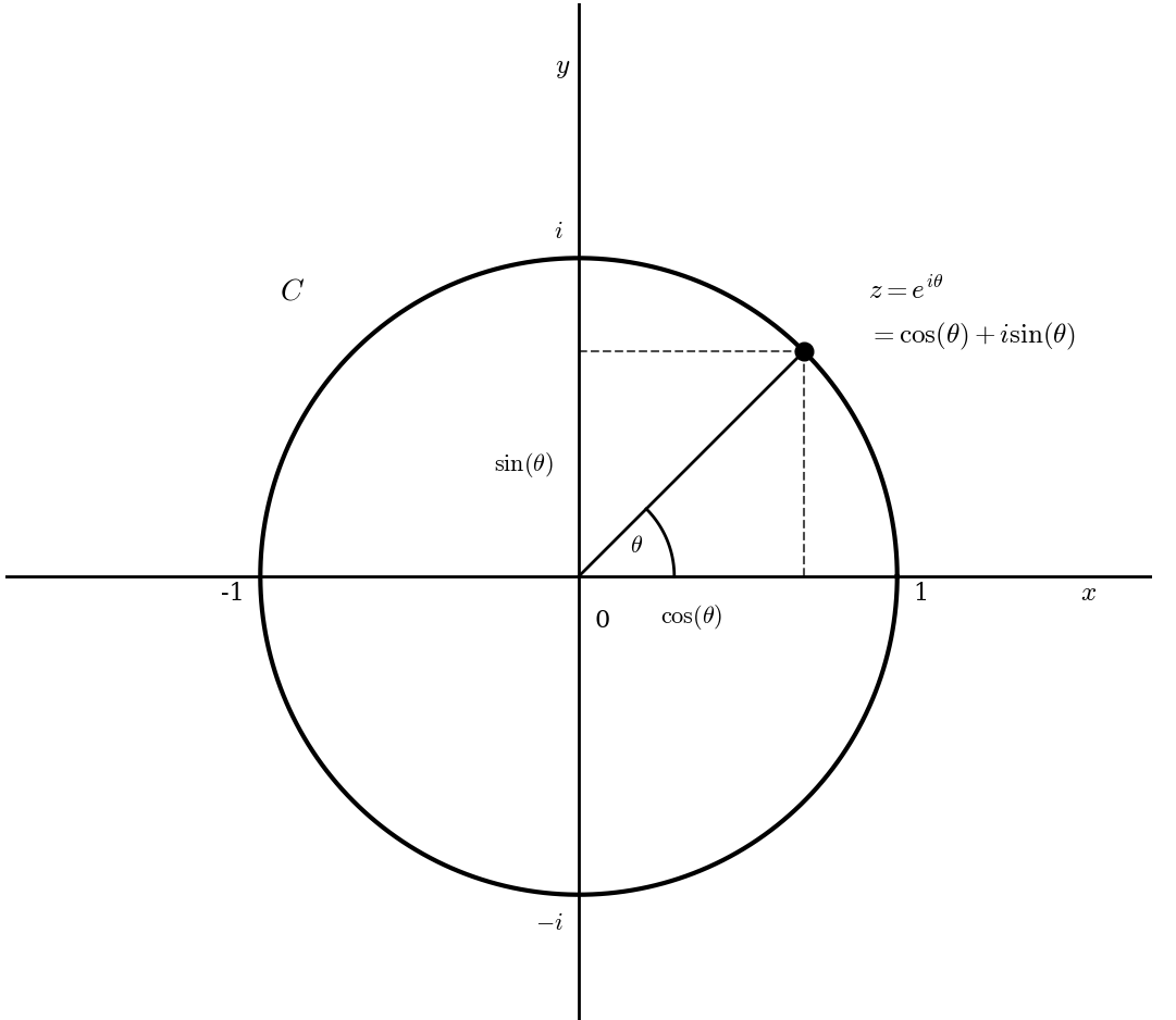
Let’s use the simplest and most convenient loop: the unit circle, parametrized by \(z = e^{i\theta}\) for \(\theta \in [-\pi, \pi]\). Let’s see what happens to our formula.
- The function is \(f(z) = h(z)^m\).
- The differential is \(dz = i e^{i\theta} d\theta\).
- The denominator is \(z^{n+1} = (e^{i\theta})^{n+1} = e^{i(n+1)\theta}\).
Plugging these in, we get: \[ \Pr(S_m=n) = \frac{1}{2\pi i} \int_{-\pi}^{\pi} \frac{h(e^{i\theta})^m}{e^{i(n+1)\theta}} (i e^{i\theta} d\theta) \] The \(i\) in the numerator cancels the \(i\) in the denominator. The \(e^{i\theta}\) from \(dz\) cancels one power in the denominator, changing \(e^{i(n+1)\theta}\) to \(e^{in\theta}\). The expression simplifies to: \[ \Pr(S_m=n) = \frac{1}{2\pi} \int_{-\pi}^{\pi} h(e^{i\theta})^m e^{-in\theta} d\theta \] Wait a minute… that’s amazing! This is exactly the formula for the \(n\)-th coefficient of a Fourier series!
A Deep Connection: Power Series and Fourier Series
Why did this happen? This is not a coincidence, it’s one of the most beautiful connections in mathematics. It’s about changing our point of view.
- A Power Series (like our PGF) is built on a basis of monomials: \(\{1, z, z^2, z^3, \dots\}\). These are simple algebraic objects.
- A Fourier Series is built on a basis of complex exponentials: \(\{\dots, e^{-2i\theta}, e^{-i\theta}, 1, e^{i\theta}, e^{2i\theta}, \dots\}\). These are functions of pure oscillation.
When we evaluate our PGF on the unit circle by setting \(z=e^{i\theta}\), we are swapping out the algebraic basis for the oscillation basis. The power \(z^k\) becomes the pure frequency \(e^{ik\theta}\).
The integral in Cauchy’s formula is a machine for extracting coefficients by averaging over a circular path. The integral in Fourier analysis is a machine for extracting coefficients by evaluating a dot product with a specific frequency (projecting onto the basis function). It turns out they are the same machine! The act of choosing the unit circle as our path in the complex plane forces the coefficient-extractor to behave just like a Fourier component-extractor.
Analyzing the Integral with a Taylor Series
To analyze the result of the above mentioned integral properly, we must approximate it for large \(m\).
The “Characteristic Function” Appears Out of Nowhere!
A natural question is: why not expand \(h(e^{i\theta})^m\) directly? A function raised to a large power \(m\) is mathematically very difficult to handle. The standard and most powerful technique is to first analyze its logarithm. This clever step turns the difficult power \(m\) into a simple multiplier.
So let’s look closely at the thing we’re taking the log of: \(h(e^{i\theta})\). What is it really? Let’s write it out: \[ h(e^{i\theta}) = \sum_k \Pr(X=k) e^{ik\theta} \] This is a sum where each possible outcome’s complex exponential \(e^{ik\theta}\) is weighted by its probability. This is just the expected value of the complex random variable \(e^{i\theta X}\)! \[ h(e^{i\theta}) = \mathbb{E}[e^{i\theta X}] \] This object is so important in probability theory that it has its own name: the Characteristic Function, denoted \(\varphi_X(\theta)\).
This is crucial. In many academic books, the characteristic function is introduced on page one like a rabbit pulled from a hat, leaving us wondering where it came from. But here, this isn’t the case at all! It has emerged completely naturally. We started with the intuitive idea of a PGF for counting. We then used a complex analysis machine to extract a coefficient. By running that machine on the unit circle, the PGF automatically transformed itself into the characteristic function. It’s the Fourier transform of the probability distribution, and it appears because we chose a Fourier-like method to solve our problem. Isn’t this cool?
So, we define \(g(\theta) = \log \varphi_X(\theta) = \log h(e^{i\theta})\). Our integrand’s exponent is now \(m\, g(\theta) - in\theta\).
The Taylor Series and Cumulants
The natural next step to approximate the integral is to expand the function \(g(\theta)\) as a Taylor series. This immediately raises the important question: around which point should we center the expansion? As we will see, the entire success of the approximation hinges on choosing \(\theta=0\).
The rigorous answer for this choice lies in analyzing the magnitude of our integrand. The integral we must solve is \(\frac{1}{2\pi} \int \varphi_X(\theta)^m e^{-in\theta} d\theta\). The dominant term that dictates the behavior of the integral for large \(m\) is \(\varphi_X(\theta)^m\). To analyze its magnitude, we use a key property of complex numbers: the magnitude of a number raised to a power is the magnitude of the number raised to that same power, i.e., \(|z^n|=|z|^n\). Therefore, the magnitude of our term is simply \(|\varphi_X(\theta)|^m\).
Our first step is to prove that the magnitude of the characteristic function, \(|\varphi_X(\theta)|\), is at most \(1\). The intuition for this comes from visualizing the sum of complex numbers as vector addition—since complex numbers add component-wise, just like vectors, the process can be seen as joining vectors tip-to-tail. The triangle inequality (\(|\sum z_i| \le \sum |z_i|\)) simply states that the length of the final resulting vector can never be greater than the sum of the lengths of all the individual vectors.
By definition, \(\varphi_X(\theta) = \sum_k p_k e^{ik\theta}\). Applying the triangle inequality: \[ |\varphi_X(\theta)| = \left|\sum_k p_k e^{ik\theta}\right| \le \sum_k |p_k e^{ik\theta}| = \sum_k p_k |e^{ik\theta}| \] Since \(|e^{ik\theta}|=1\) for any real \(k\) and \(\theta\), this simplifies to: \[ |\varphi_X(\theta)| \le \sum_k p_k = 1 \] The equality \(|\varphi_X(\theta)|=1\) holds if and only if all the complex numbers \(e^{ik\theta}\) (for which \(p_k>0\)) point in the same direction. For any non-trivial distribution (with at least two different outcomes), this only happens when \(\theta=0\). At \(\theta=0\), every term \(e^{ik\cdot 0}\) is just 1. For any \(\theta \neq 0\), the different values of \(k\) cause the terms to have different phases, so they are no longer perfectly aligned, and the magnitude of their sum is strictly less than 1. This means that the function \(|\varphi_X(\theta)|\) has a unique, global maximum value of 1 at precisely \(\theta=0\).
Now, consider what happens when we raise this to a large power, \(m\). The peak at \(\theta=0\), where the value is \(1^m = 1\), remains. However, for any other value of \(\theta\) where \(|\varphi_X(\theta)| < 1\), the value of \(|\varphi_X(\theta)|^m\) plummets towards zero exponentially fast as \(m\) grows. For instance, if at some point the magnitude is 0.99, for \(m=1000\) it becomes \(0.99^{1000} \approx 4 \times 10^{-5}\).
This creates a very sharp “spike” in the integrand’s magnitude, centered at \(\theta=0\). The result is that the only part of the integral that contributes significantly to the final value comes from an infinitesimally small neighborhood around \(\theta=0\). The contributions from all other regions are exponentially suppressed and become negligible. Therefore, to accurately approximate the integral for large \(m\), we must approximate the function \(g(\theta)\) in this tiny but important region around the origin. The Taylor series is the fundamental for this. Expanding around \(\theta=0\) is not a mere convenience; it is a necessary step.
Now that we have established why we must expand around \(\theta=0\), we can proceed further. The Taylor series of \(g(\theta) = \log \mathbb{E}[e^{i\theta X}]\) is special because its coefficients define the cumulants (\(\kappa_j\)) of our distribution. The general formula for the \(j\)-th cumulant is given by the \(j\)-th derivative of the log-generating function evaluated at the origin: \[ \kappa_j = \frac{1}{i^j} \left. \frac{d^j}{d\theta^j} \, g(\theta) \right|_{\theta=0}. \]
These cumulants are the distribution’s fundamental properties:
- \(\kappa_1 = \mu\) (the mean)
- \(\kappa_2 = \sigma^2\) (the variance)
- \(\kappa_3 = \mathbb{E}[(X-\mu)^3]\) (the third central moment, a measure of skewness)
- \(\kappa_4 = \mathbb{E}[(X-\mu)^4] - 3(\sigma^2)^2\) (related to kurtosis)
The Taylor series of \(g(\theta)\) around \(\theta=0\) (assuming the corresponding moments exist) is therefore:
\[ g(\theta) = i\mu\,\theta - \frac{\sigma^2}{2}\,\theta^2 - i\,\frac{\kappa_3}{6}\,\theta^3 + \frac{\kappa_4}{24}\,\theta^4 + O(\theta^5). \]
The Bell Curve Emerges
Setting the Stage
Now we put our Taylor series approximation back into the integral for \(\Pr(S_m=n)\). The exponent in our integral, \(m\, g(\theta) - in\theta\), becomes: \[ m\left(i\mu\,\theta - \frac{\sigma^2}{2}\,\theta^2 - i\frac{\kappa_3}{6}\,\theta^3 + \frac{\kappa_4}{24}\,\theta^4 + \dots\right) - in\theta. \] This still looks like a complicated mess. The key insight is that for large \(m\), the sum \(S_m\) will almost certainly be very close to its expected value, \(m\mu\). We are interested in the shape of the distribution around this mean. The question “what does the distribution of the sum look like?” is really “what does the distribution of deviations from the mean look like?”
To formalize this, we need a new coordinate system that is centered at the mean and scaled appropriately. The mean of the sum \(S_m\) is \(m\mu\), and its variance is \(m\sigma^2\), making its standard deviation \(\sigma\sqrt{m}\). It is natural to measure deviations in units of this standard deviation.
So, we define a new variable \(x\) that does exactly this: \[ n = m\mu + x\sigma\sqrt{m} \] Here, \(x\) is our new coordinate, representing the number of standard deviations from the mean. An \(x\) value of 0 is the mean, \(x=1\) is one standard deviation above the mean, and so on. This change of variables is not just a trick; it is the fundamental act of standardizing the random variable so we can compare the shapes of distributions that have different means and variances.
Let’s substitute this into our exponent: \[ m\left(i\mu\,\theta - \frac{\sigma^2}{2}\,\theta^2 - \dots\right) - i(m\mu + x\sigma\sqrt{m})\theta \] Distributing the last term gives: \[ (im\mu\theta - m\frac{\sigma^2}{2}\theta^2 - \dots) - im\mu\theta - ix\sigma\sqrt{m}\theta \] Look! The main term involving the mean, \(im\mu\theta\), cancels out perfectly! This is no accident; this is why we centered our coordinate system at the mean. The purpose of this step was to eliminate the shifting effect of the mean so we could focus purely on the shape of the distribution. The exponent becomes: \[ -m\frac{\sigma^2}{2}\theta^2 - ix\sigma\sqrt{m}\theta - m\left(i\frac{\kappa_3}{6}\theta^3 + \dots\right) \]
A Mathematical Microscope
Our exponent, \(-m\frac{\sigma^2}{2}\theta^2 - ix\sigma\sqrt{m}\theta - m\left(i\frac{\kappa_3}{6}\theta^3 + \dots\right)\), still looks complicated. The key to simplifying it is to understand the behavior for large \(m\).
The term \(e^{-m\frac{\sigma^2}{2}\theta^2}\) acts as a Gaussian “envelope” that rapidly decays to zero as \(\theta\) moves away from the origin. As \(m\) gets larger, this envelope shrinks tighter and tighter, meaning the effective region of integration gets narrower. This provides a reason for our earlier insight: the integral is dominated by the behavior near \(\theta=0\).
This observation forces a critical question: how do we properly “zoom in” on the origin to see the stable, non-trivial behavior of the integral as \(m \to \infty\)? We need a change of variables for \(\theta\) that depends on \(m\). Let’s consider the dominant term, \(m\theta^2\). For the integral to converge to a meaningful, constant shape, this term must be stable — it cannot vanish or diverge as \(m \to \infty\). This implies that \(m\theta^2\) must be of order \(1\). This simple requirement dictates the scaling: \[ m\theta^2 \sim \text{constant} \implies \theta \sim \frac{1}{\sqrt{m}} \] This is the unique scaling that works. If we zoomed in too much (e.g., \(\theta \sim 1/m\)), the quadratic term would vanish and we’d lose the Gaussian shape. If we didn’t zoom in enough (e.g., \(\theta \sim 1/m^{1/4}\)), the term would blow up.
This insight motivates the formal change of variables: \[ \theta = \frac{u}{\sqrt{m}} \] Here, \(u\) is our new coordinate, a “stabilized” variable that lives on a constant scale while we send \(m \to \infty\). This change of variables is like placing the integrand under a mathematical microscope with a zoom level of \(\sqrt{m}\), perfectly calibrated to reveal the universal shape hidden at the origin. It is important to remember that this is a standard change of variables for a definite integral. We are simply re-scaling our axis of integration; the value of the integral is preserved as long as we correctly transform the differential (\(d\theta = du/\sqrt{m}\)) and the integration limits. Let’s see why this is perfect by examining each term in the exponent:
The Variance Term: \[ -m\frac{\sigma^2}{2}\theta^2 \quad \longrightarrow \quad -m\frac{\sigma^2}{2}\left(\frac{u}{\sqrt{m}}\right)^2 = -m\frac{\sigma^2}{2}\frac{u^2}{m} = -\frac{\sigma^2}{2}u^2 \] The \(m\) vanishes completely! This term becomes independent of \(m\), forming the stable, universal core of our bell curve. This is the main event.
The \(x\) Term (from centering): \[ -ix\sigma\sqrt{m}\theta \quad \longrightarrow \quad -ix\sigma\sqrt{m}\left(\frac{u}{\sqrt{m}}\right) = -ix\sigma u \] This term is also stable and independent of \(m\). It controls the position under the bell curve.
The Skewness Term (\(\kappa_3\)): \[ -m\left(i\frac{\kappa_3}{6}\theta^3\right) \quad \longrightarrow \quad -mi\frac{\kappa_3}{6}\left(\frac{u}{\sqrt{m}}\right)^3 = -mi\frac{\kappa_3}{6}\frac{u^3}{m^{3/2}} = -i\frac{\kappa_3 u^3}{6\sqrt{m}} \] This term has a \(\sqrt{m}\) in the denominator, so it vanishes as \(m \to \infty\)!
The Kurtosis Term (\(\kappa_4\)): \[ m\left(\frac{\kappa_4}{24}\theta^4\right) \quad \longrightarrow \quad m\frac{\kappa_4}{24}\left(\frac{u}{\sqrt{m}}\right)^4 = \frac{\kappa_4 u^4}{24 m} \] This is smaller, of order \(m^{-1}\), and contributes to higher-order accuracy (e.g., beyond the first Edgeworth correction).
Higher-Order Terms: All subsequent terms will have even higher powers of \(\sqrt{m}\) in the denominator (\(m, m^{3/2}, \dots\)), so they will disappear even faster.
Our once messy exponent simplifies beautifully: \[ \text{Exponent} = \underbrace{-\frac{\sigma^2}{2}u^2 - ix\sigma u}_{\text{The stable Bell Curve shape}} \; - \; \frac{i\kappa_3 u^3}{6\sqrt{m}} \; + \; \frac{\kappa_4 u^4}{24 m} \; + \; O\!\left(m^{-3/2}\right) \] As \(m \to \infty\), all the terms that depend on the specific, unique features of our original die (skewness, kurtosis, etc.) are washed away. Only the terms related to the mean and variance survive.
Our integral for the probability becomes: \[ \Pr(S_m=n) \approx \frac{1}{2\pi} \int \exp\left(-\frac{\sigma^2 u^2}{2} - ix\sigma u\right) (du/\sqrt{m}) \] The change of variables \(d\theta = du/\sqrt{m}\) introduces the \(\frac{1}{\sqrt{m}}\) factor. The integral is now over \(u\). Since the integrand shrinks to zero incredibly fast for large \(u\), we can extend the limits of integration from \([-\pi\sqrt{m}, \pi\sqrt{m}]\) to \([-\infty, \infty]\) with negligible error. \[ \Pr(S_m=n) \approx \frac{1}{2\pi\sqrt{m}} \int_{-\infty}^{\infty} \exp\!\left(-\frac{\sigma^2 u^2}{2} - ix\sigma u\right) \, du. \]
Evaluating the Gaussian Integral and Finding the PDF
This is a standard Gaussian integral. We can solve it by completing the square in the exponent: \[ -\frac{\sigma^2 u^2}{2} - ix\sigma u = -\frac{\sigma^2}{2}\left(u^2 + \frac{2ix}{\sigma}u\right) = -\frac{\sigma^2}{2}\left(\left(u + \frac{ix}{\sigma}\right)^2 - \left(\frac{ix}{\sigma}\right)^2\right) = -\frac{\sigma^2}{2}\left(u + \frac{ix}{\sigma}\right)^2 - \frac{x^2}{2} \] The integral becomes: \[ \int_{-\infty}^{\infty} e^{-\frac{\sigma^2}{2}(u + ix/\sigma)^2 - x^2/2} du = e^{-x^2/2} \int_{-\infty}^{\infty} e^{-\frac{\sigma^2}{2}(u + ix/\sigma)^2} du \] The integral on the right-hand side is a form of the Gaussian integral. Its evaluation hinges on a key property: an integral of the form \(\int_{-\infty}^{\infty} e^{-a(t+b)^2}dt\) is equal to \(\sqrt{\pi/a}\), regardless of the shift \(b\) (for a beautiful derivation of this integral, see 3Blue1Brown here).
If \(b\) is a real number, this is easy to see. We can just make a substitution \(u = t+b\). Then \(du = dt\), and the limits of integration don’t change. The integral becomes \(\int_{-\infty}^{\infty} e^{-au^2}du\), which is a standard Gaussian integral whose value is \(\sqrt{\pi/a}\).
In our case, the shift is a purely imaginary number (\(b = ix/\sigma\)). This makes the substitution a bit more subtle, as it shifts the path of integration off the real axis and into the complex plane. The full justification comes from a result in complex analysis called Cauchy’s Integral Theorem, which states that for a “well-behaved” function (analytic) like our integrand, the integral’s value doesn’t change when we shift the integration contour, provided we don’t cross any singularities (which our function doesn’t have).
So, whether the shift \(b\) is real or complex, the result is the same. For our integral, we have \(a=\sigma^2/2\), so the integral evaluates to \(\sqrt{\pi/(\sigma^2/2)} = \sqrt{2\pi/\sigma^2}\).
Plugging this back in: \[ \Pr(S_m=n) \approx \frac{1}{2\pi\sqrt{m}} \cdot \sqrt{\frac{2\pi}{\sigma^2}} e^{-x^2/2} = \frac{1}{\sigma\sqrt{2\pi m}} e^{-x^2/2}. \] This is the Local Limit Theorem. It gives the probability of a single outcome. But what does it represent? Let’s rearrange it. The quantity \(1/(\sigma\sqrt{m})\) is the spacing between possible values of our standardized variable \(x\). Let’s call this spacing \(\Delta x\). Then \[ \Pr(S_m=n) \approx \frac{1}{\sqrt{2\pi}} e^{-x^2/2} \cdot \frac{1}{\sigma\sqrt{m}} = \frac{1}{\sqrt{2\pi}} e^{-x^2/2} \Delta x. \] This is beautiful! It says that the probability of landing in a small interval of width \(\Delta x\) around the value \(x\) is approximately the height of a curve, \(\frac{1}{\sqrt{2\pi}} e^{-x^2/2}\), times the width of the interval. This is the definition of a probability density function!
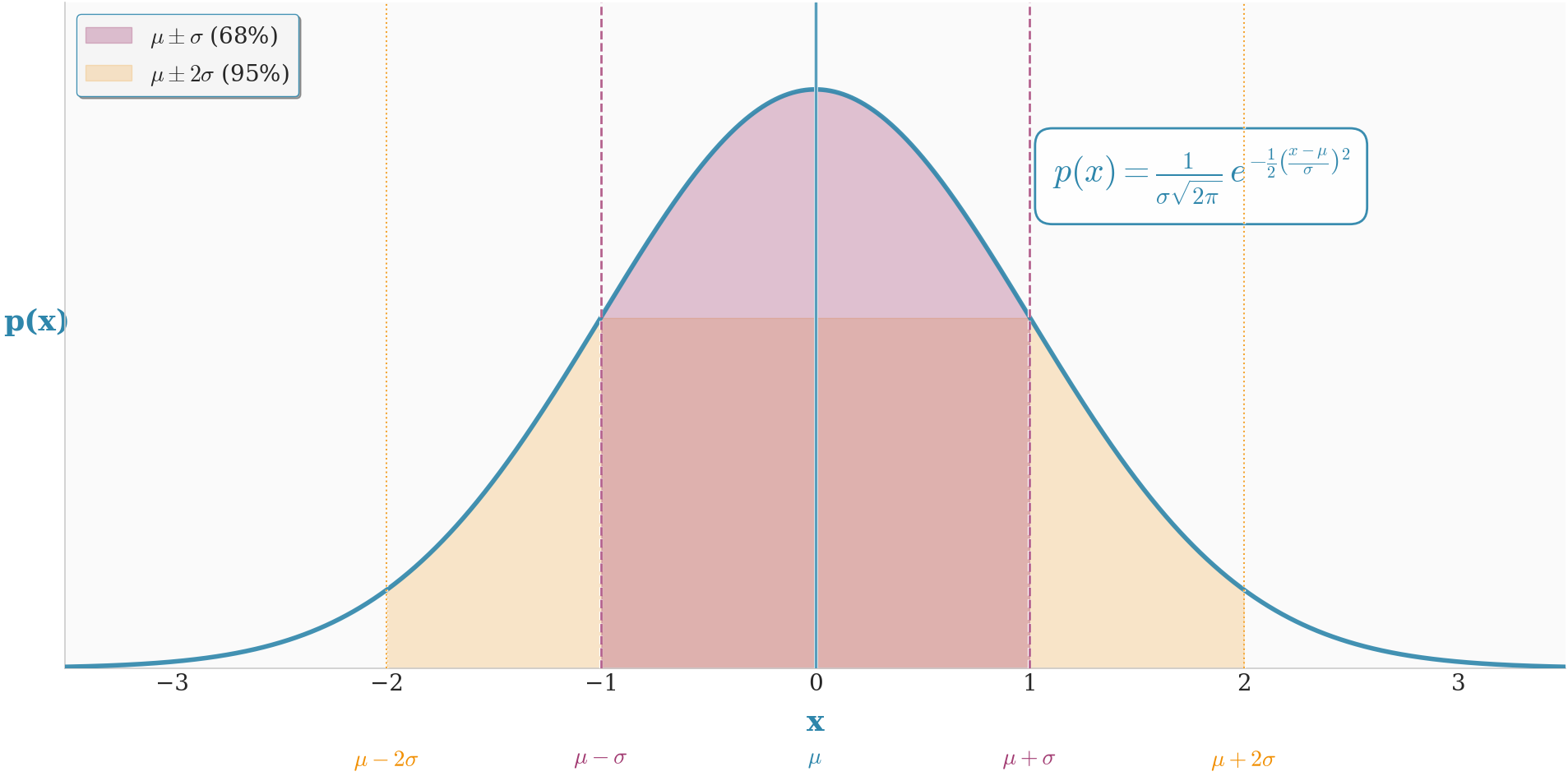
As \(m\to\infty\), the discrete steps \(\Delta x\) become infinitesimally small, and the approximation becomes exact. We have just derived the probability density function (PDF) of the standardized normal distribution: \[ f(x) = \frac{1}{\sqrt{2\pi}} e^{-x^2/2} \] The mean and variance of the original distribution are hidden in here. The mean \(\mu\) was removed when we centered our variable \(x\). The variance \(\sigma^2\) was scaled away to give this universal shape. This shows that any sum of i.i.d. variables, when recentered and rescaled, will converge to this exact same shape.
A Sharper Approximation: The Edgeworth Correction
What if we keep the next term in the exponent? \[ e^{\text{Exponent}} \approx e^{-\frac{\sigma^2 u^2}{2} - ix\sigma u} \cdot e^{-i\frac{\kappa_3 u^3}{6\sqrt{m}}} \] For large \(m\), the argument of the second exponential is small, so we can use the approximation \(e^y \approx 1+y\): \[ e^{-\frac{\sigma^2 u^2}{2} - ix\sigma u} \left(1 - i\frac{\kappa_3 u^3}{6\sqrt{m}}\right) \] Integrating this gives the main Gaussian term plus a correction term involving the integral of \(u^3\) against the Gaussian. The result is the first-order Edgeworth series expansion: \[ \Pr(S_m=n) \approx \frac{1}{\sigma\sqrt{2\pi m}} e^{-x^2/2} \left[1 + \frac{\kappa_3}{6\,\sigma^3\,\sqrt{m}}(x^3-3x)\right]. \] This correction term accounts for the skewness (\(\kappa_3\)) of the original distribution, and it’s our first hint of how the sum approaches the bell curve, along with the shape of the errors in the approximation.
Beyond integer-valued variables (real-valued \(X\))
So far, our random variable \(X\) could only take integer values. What if it’s a continuous variable that can take any real value? We can cleverly handle this by thinking of a continuous value as a limit of finely-grained discrete values.
Let’s imagine a continuous random variable \(X\) with some probability density function. We can approximate it with a discrete variable \(X_N\) that takes values on a fine grid with spacing \(1/N\): \(k/N\) for integers \(k\). The probability that \(X_N\) takes the value \(k/N\) would be approximately the density of \(X\) at that point times the spacing: \(\Pr(X_N = k/N) \approx f(k/N) \cdot (1/N)\).
Now, we can build a PGF for this discretized variable \(X_N\). But the powers will be fractions, like \(z^{k/N}\). This looks strange, but we can make it familiar with a simple substitution. Let a new variable be \(\zeta = z^{1/N}\). Then our PGF becomes a normal polynomial (or Laurent series) in \(\zeta\): \[ H_N(\zeta) = \sum_k \Pr(X_N = k/N) \zeta^k \] This is amazing! We’ve transformed the continuous problem back into the discrete integer problem we just solved. We can now use our entire machinery on this new PGF.
The sum of \(m\) such independent variables, \(S_m = X_{N,1} + \dots + X_{N,m}\), will have a PGF of \(H_N(\zeta)^m\). The probability that this sum equals a certain value, say \(n/N\), is given by the coefficient of \(\zeta^n\): \[ \Pr(S_m = n/N) = [\zeta^n]H_N(\zeta)^m \] We can run this through our whole derivation. The mean and variance of \(X_N\) will be approximately the mean and variance of \(X\), and as we take the limit \(N \to \infty\), they will become exact. The final result for the probability will look just like our Local Limit Theorem, but for the variable \(\zeta\).
When we translate back, we find that the probability density function of the sum \(S_m\) converges to the same bell curve shape. The insight is that the underlying logic — convolution becoming multiplication, logarithms linearizing powers, and the dominance of the quadratic term in the Taylor series — is completely independent of whether the original variable was discrete or continuous. By discretizing, we can see that the same universal force is at play. The passage to the continuous case is just a matter of taking the limit as our grid becomes infinitely fine. This confirms that the CLT is a universal law of probability.